Useful libraries for scientific computing

One of the strongest points of Python is the flourishing ecosystem of libraries it comes with. We have already seen some of them, such as numpy and matplotlib. This chapter reviews other libraries that are handy to code scientific computing applications, including computational chemistry ones. We will mostly focus on scipy, highlighting some of its submodules that provide a huge set of numerical algorithms, and also briefly mention other projects that you will likely find useful. The classification of these libraries as integral components of Python’s core or specialized tools might provoke debate, yet you’ll undoubtedly benefit from the diverse array of supplementary features accessible across various layers.

scipy

This module contains a collection of numerical algorithms such as integration, optimization, interpolation, linear algebra, statistics, and much more. It is built on top of numpy, i.e., it mainly uses numpy arrays as the main data structure.

scipy is organized in submodules, each one with a specific purpose, which can be imported separately as,

import scipy.submodulename
#or
from scipy import submodulename

The submodules that normally fulfill the needs of a computational chemist are:

• integrate: Integration and ordinary differential equation solvers

• interpolate: Interpolation and smoothing splines

• optimize: Optimization and root-finding routines

• linalg: Linear algebra, which actually provides an interface to BLAS and LAPACK libraries. Note that it generally supports all numpy.linalg functions, and scipy.linalg versions are preferred.

In this chapter we will focus on the first three submodules. The list of submodules is more extensive, including fft (Fast Fourier Transform), special (special functions, such as Hermite polynomials). A complete list can be found in the official documentation.

scipy.integrate

This submodule provides several integration routines, including an ordinary differential equation integrator.

Integration of a 1D function, can be done with the quad method. It takes a function and the integration limits as arguments, and returns the integral and an estimate of the error. Let’s see an example:

from scipy.integrate import quad
import numpy as np

def gaussian(x, mu, sigma):
    return 1/np.sqrt(2*np.pi*sigma**2)*np.exp(-(x-mu)**2/(2*sigma**2))

mu = 0
sigma = 1
norm, err = quad(gaussian, -np.inf, np.inf, args=(mu, sigma))
print(norm)

0.9999999999999997

Other methods to integrated 1D functions are fixed_quad, quadrature or romberg.

Instead, integration of a discrete function (1D), i.e., a set of points, can be done with the trapz, romb and simps functions. In the case, the functions take as arguments the x and y arrays with the grid and function values, and return the integral. For instance,

from scipy.integrate import simps
import numpy as np

def gaussian(x, mu, sigma):
    return 1/np.sqrt(2*np.pi*sigma**2)*np.exp(-(x-mu)**2/(2*sigma**2))

x = np.linspace(-100, 100, 5000)
mu = 0
sigma = 1
y = gaussian(x, mu, sigma)
print(simps(y, x=x))

1.0000000000000002

Exercise

Write a program to check the orthogonality of the vibrational eigenfunctions of the harmonic oscillator.

Hint: The eigenfunctions of the harmonic oscillator can be written as:

\[ \psi_n(Q) = \frac{1}{\sqrt{2^n n!}} \left(\frac{\omega}{\pi\hbar}\right)^{1/4} e^{-\omega Q^2/2\hbar} H_n\left(\sqrt{\frac{\omega}{\hbar}}Q\right) \]

where \(H_n\) are the Hermite polynomials, which can be evaluated with the function scipy.special.eval_hermite.

Functions for multidimensional integration are also available, such as dblquad (double integral), tplquad (triple integral) and nquad (integration over multiple variables).

This submodule also provides methods to integrate ordinary differential equations. The recommended method is solve_ivp (solve initial value problem), which gives an interface to different integration algorithms. For instance, in order to integrate the system of differential equations below,

\[\begin{split} \begin{align} \frac{dx}{dt} &= -y \\ \frac{dy}{dt} &= x \end{align} \end{split}\]

we can use the following code,

from scipy.integrate import solve_ivp
import numpy as np
import matplotlib.pyplot as plt

def f(t, y):
    return [-y[1], y[0]]
    
t0 = 0
tf = 10
y0 = [1, 0]
t_eval = np.linspace(t0, tf, 100)
sol = solve_ivp(f, [t0, tf], y0, t_eval=t_eval)

plt.plot(sol.t, sol.y[0], label='x')
plt.plot(sol.t, sol.y[1], label='y')
plt.legend()
plt.show()

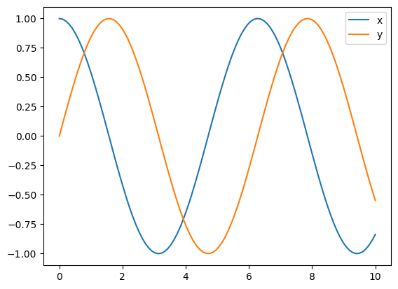
The integration algorithm is set with the method attribute, with the default being RK45 (Runge-Kutta of 4th order).

scipy.interpolate

This submodule provides several interpolation routines. In the case of 1D interpolation, i.e. from a discrete set of \((x,y)\) points, the most common method is interp1d. This function takes as arguments the x and y arrays, and returns a function object that can be evaluated at any point, within the range of x (values out of this range can be managed with the fill_value argument). For instance,

from scipy.interpolate import interp1d
import numpy as np
import matplotlib.pyplot as plt

x = np.linspace(0, 10, 10)
y = np.sin(x)
f = interp1d(x, y, kind='cubic')

xnew = np.linspace(0, 10, 100)
ynew = f(xnew)

plt.plot(x, y, 'o', xnew, ynew, '-')
plt.show()

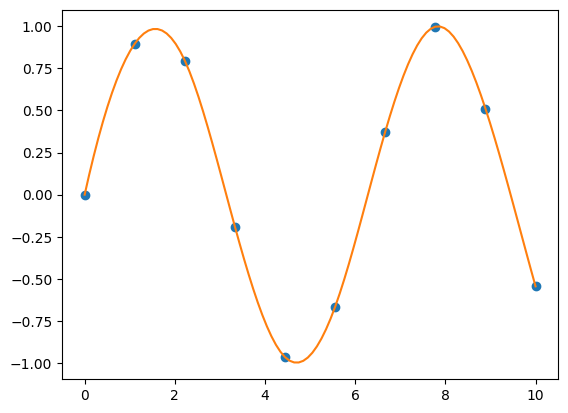
As shown in the above example, the kind argument specifies the type of interpolation. Possible values include linear (which is the default), quadratic or cubic (a complete list can be found in the official documentation).

Exercise

Write a program that sums two spectra defined over different wavelength ranges. Use interpolation to generate a common wavelength grid, and then sum the spectra.

Note: spectra to test your code can be obtained from PhotochemCAD. You can use the requests module to download the files:

import requests

# Azobenzene
URL = "https://omlc.org/spectra/PhotochemCAD/data/117-abs.txt"
response = requests.get(URL)
open("spc1.dat", "w").write(response.content)

# 9,10-Diphenylanthracene
URL = "https://omlc.org/spectra/PhotochemCAD/data/021-abs.txt"
response = requests.get(URL)
open("spc2.dat", "w").write(response.content)

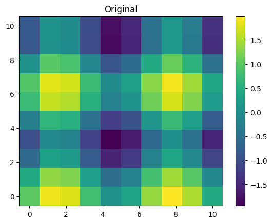
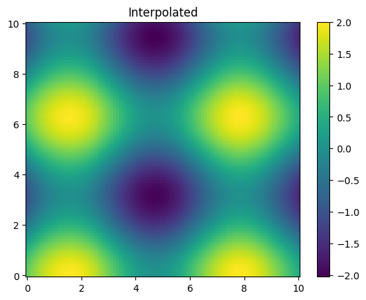
For 2D interpolation, the most general function is interp2d. This function takes as arguments a 2D array of values, Z, and the two 1D arrays of coordinates, x and y. These arrays do not have to be equally spaced. As in the 1D case, it returns a function that can be evaluated at any point.

from scipy.interpolate import interp2d
import numpy as np
import matplotlib.pyplot as plt

x = np.linspace(0, 10, 10)
y = np.linspace(0, 10, 10)
X, Y = np.meshgrid(x, y)
Z = np.sin(X) + np.cos(Y)

f = interp2d(x, y, Z, kind='cubic')

xnew = np.linspace(0, 10, 100)
ynew = np.linspace(0, 10, 100)
znew = f(xnew, ynew)

plt.pcolormesh(X, Y, Z)
plt.colorbar()
plt.title('Original')
plt.show()
plt.pcolormesh(xnew, ynew, znew)
plt.colorbar()
plt.title('Interpolated')
plt.show()

As you can see, we use some kind of advanced matplotlib features in this example. You can refresh them going back to the previous chapter. For instance, use the np.meshgrid function, which generates 2D arrays with the grid points, (x,y), from the corresponding 1D arrays, x and y. The interpolation method is specified with the kind argument, which can take the same values as in the 1D case.

The above example uses a regular grid, but this is not a requirement. Actually, in this case we can use the function RectBivariateSpline, which is more efficient but is restricted to regular grids. This function takes the same arguments as interp2d.

To interpolate unstructured data we can use the function griddata. It takes as arguments the coordinates of the data points as a tuple of 1D arrays, (x,y) and the values at these points, z, also a 1D array. It also takes the coordinates of the points where the interpolation is required, (Xi,Yi). In this case, it returns the interpolated values at these points as a 2D array Zi. The interpolation method is specified with the method argument. Possible values are linear, nearest and cubic.

scipy.optimize

This module provides several algorithms for optimization (locating minima and maxima) and root-finding.

The function minimize provides a common interface to all the optimization algorithms. It takes as arguments the function to be minimized, f(x), the initial guess, x0, and the method to be used, method. The function to be minimized must take as argument a 1D array with the values of the variables to be optimized, and return a scalar. For instance,

from scipy.optimize import minimize
import numpy as np

def f(x):
    return np.sum(x**2)
    
x0 = np.array([1, 2, 3])
res = minimize(f, x0, method='Nelder-Mead')
print(res.x)

[-4.80659631e-05 -1.10944154e-05 -1.86599703e-05]

As shown above, the minimize function returns an object with the results of the optimization. The x attribute contains the values of the variables that minimize the function. Other attributes of the result object are fun, which contains the value of the function at the minimum, success, which is a boolean indicating if the optimization was successful, or the number of iterations, nit, among others.

Different optimization algorithms can be used with the method argument, including BFGS (default for unconstrained problems) or Newton-CG. The choice of the method depends on the problem (stiffness, dimensionality, etc.), and the need of adding constraints A complete list is given in the documentation.

For root-finding of scalar functions (univariate functions, i.e., which depend on only one variable), we can use the general interface function root_scalar. It takes as arguments the function to be solved, f(x) and some other arguments depending on the method to be used, method. For instance, with method=bisect, we need to provide the closed interval where the solution lies, bracket. Other methods may require the derivative of the function, fprime and/or an initial guess, x0. The function to be solved must take as argument a scalar and return a scalar. For instance,

from scipy.optimize import root_scalar
import numpy as np

def f(x):
    return np.exp(x) + x
    
res = root_scalar(f, bracket=[-2.0,2.0], method='bisect')
print(res.root)

-0.5671432904109679

Again, the root_scalar function returns an object with the results of the root-finding. The root attribute contains the value of the variable that solves the equation.

The function root provides a common interface to all the root-finding algorithms for vector functions (i.e, a system of N equations that depend on N variables). It takes as arguments the function to be solved, f(x), which depends on a 1D array (vector) of N variables, x, the initial guess, x0, and the method to be used, method. The function to be solved must take as argument a 1D array with the values of the variables to be solved, and returns a 1D array with the same shape. For instance, the following system of equations:

\[\begin{split} \begin{align} x^2 + y^2 = 1 \\ x - y = 0 \end{align} \end{split}\]

can be solved as follows:

from scipy.optimize import root
import numpy as np

def f(x):
    return np.array([x[0]**2 + x[1]**2 - 1, x[0] - x[1]])

x0 = np.array([1, 2])
res = root(f, x0, method='hybr')
print(res.x)

[0.70710678 0.70710678]

Available methods are summarized in the documentation of this function.

sympy

This module is a computer algebra system (CAS), similar to Maxima or Mathematica. It allows performing symbolic calculations, such as derivatives, integrals, solving equations, etc.

We will not go into details here, but we will show some examples of the capabilities of this module. For instance, lets compute the derivative of the function \(f(x) = \sin(x) \cos(x)\):

from sympy import symbols, sin, cos, diff

x = symbols('x')
f = sin(x)*cos(x)
df = diff(f, x)
df

\[\displaystyle - \sin^{2}{\left(x \right)} + \cos^{2}{\left(x \right)}\]

Many other symbolic operations are possible, such as integrals, limits, series expansions, etc. Check the documentation for more details.

pandas

This module provides high-performance, easy-to-use data structures and data analysis tools, allowing to manipulate and analyze large amounts of data. You can read and write data sets from file formats such as csv, excel, hdf5, etc. For instance, to read a csv file:

import pandas as pd

# Read a csv file
df = pd.read_csv('file.csv')
# Get the values of column labelled 'Col1' as a numpy array
x = df['Col1'].values

You can check the documentation for more details.

ase

ASE stands for Atomic Simulation Environment. This module provides a set of tools for setting up, manipulating, running, visualizing and analyzing atomistic simulations. It supports many codes through the Calculator interface, e.g. Gaussian or Gromacs, allowing to perform a wide range of calculations from a single Python script.

It also provides functions to read and write files in different formats (xyz, pdb…), through the ase.io submodule. For instance, to read a file in xyz format:

# The io submodule must be imported separately
import ase.io

# Generate an ASE Atom object from a file
molec = ase.io.read('file.xyz')
# Get the atomic coordinates as a numpy array:
xyz = molec.get_positions()

You can take a further look into the powerful capabilities of this library in the documentation.

h5py

This module provides support to manipulate HDF5 files, a format specifically designed to store large amounts of numerical data. There are other formats that are also very useful for this purpose, such as netCDF, JSON or XML, which are also supported by Python modules.